Tutorial: Bayesian Model Averaging with BMS under Matlab
This tutorial demonstrates the use of Bayesian Model Averaging (BMA) for a cross-section economic growth data set with the BMS toolbox for Matlab.
The lines below are partly inspired by the article Model uncertainty in cross-country growth regressions by Fernández, Ley and Steel (FLS) - however they do not fully reproduce the article but instead focuses on the available features within the toolbox.
Note that BMS toolbox for Matlab is a scaled-down derivative of the more comprehensive BMS package for R. Actually it just wraps the underlying R functions.
If you do not necessarily need Matlab for your project, or intend to do harder work, you are recommended to consider the corresponding tutorials for BMS under R.
Still, the functions in BMS toolbox for Matlab are very similar to those in the R package. The Matlab toolbox could therefore be used as well with the corresponding R tutorials.
Finally, a word of caution: Note that BMS toolbox for Matlab is still in testing phase.
Contents:
- Installing the BMS toolbox for Matlab
- Running the Bayesian Model Sampling Chain
- Interpreting the Results
- Two Concepts: Analytical Likelihoods vs. MCMC Frequencies
- Posterior Model Probabilities
- Posterior Coefficient Densities
- Advanced Topics
Installing the BMS toolbox for Matlab
In order to continue with the tutorial, you should install the toolbox, R and the linking COM-Interface according to these installation instructions.
After successful installation, open Matlab, navigate the current directory to the BMS toolbox folder 'BMS_matlab' and type:
libraryBMS;
This will open a hidden R session and add all toolbox functions to your Matlab search path.
Running the Bayesian Model Sampling Chain
Let us first load the data set of FLS, which comes along with the BMS toolbox:
load datafls;
This will load the data set in the form of a structure (Note that it could also be a Matlab dataset object, or a plain numeric matrix, such as the one resulting from load datafls_plain;).
The next step is to run Bayesian Model Averaging on this data set, with priors such as in the original FLS article. In order to save time during the demonstration, let us do fewer iterations than FLS: take 20 000 burn-ins, then 50 000 draws with the FLS sampler. And let us save the best 2000 models.
bmsGUI;
A Window will open that looks as follows:
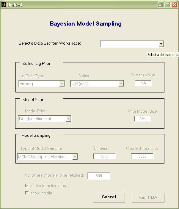
The uppermost pop-up menu lists all available data set variables in the Matlab workspace. Use it to select the variable 'datafls'.
Then choose the remaining settings as they appear in the image below.
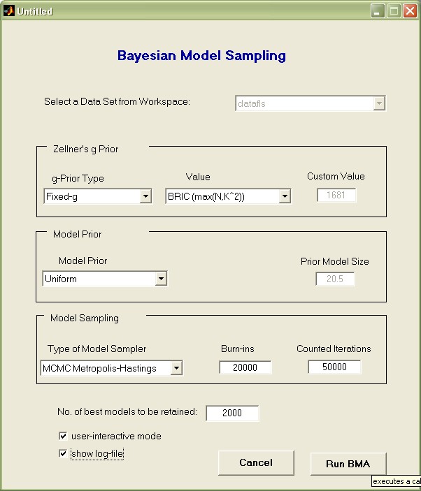
Here we chose the following settings:
- Zellner's g value: 'BRIC (max(N,K^2))' is to select the g-parameter according to the 'automatic' setting recommended by FLS
- Model Prior 'Uniform' was chosen to employ the popular uniform model prior, just as in FLS
- 'Burn-ins' was set to 20 000 initial draws (which are to be disregarded for aggregate statistics)
- The 50 000 'Counted Iterations' specify that after the 20 000 burn-ins, there should be fifty thousand draws taken into account for aggregate statistics.
- Finally, the 2 000 best models should be saved individually for more detailed analysis
Press the 'Run BMA' button: this will execute a call to the bms in the Matlab base workspace and take between 5 and 15 seconds on a modern PC.
Interpreting the Results
The call to bmsGUI put a variable named bmstemp into the workspace that represents a 'bma object'.
Moreover, it printed out results that resemble the ones provided below (any differences are due to the fact that model sampling involves random model draws and our example includes very few MCMC iterations).
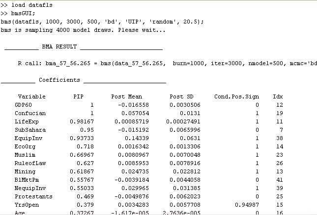
The very first line details the executed call to the function bms that would yield the same result without involving a graphical user interface (for more details, type help bms).
The section 'Coefficients' of the print-out displays the results for the explanatory variables, ordered by importance: The dummy for sub-Saharan Africa ('SubSahara'), for instance, has a posterior inclusion probability (PIP) of 95%, a posterior expected coefficient ('Post Mean') of -0.015, with a standard deviation ('Post SD') of 0.0066. A 'Cond.Pos.Sign.' of 0 shows that whenever Life Expectancy was included in a model it never had a positive (expected) coefficient.
Note that the results above can be quite unstable, as we did very few iterations for demonstration purposes.
Below the variable statistics, some general information on the BMA sampling chain is printed out, similar to the next figure:
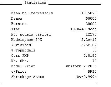
Inter alia, it shows that the posterior statistics are based on 12 273 models that were accepted by the MCMC sampler. (A more detailed explanation of the results is available by typing help summary_bma)
Note that the above information can always be retrieved from the variable bmstemp by typing the following commands:
coef_bma(bmstemp) #for the coefficients
summary_bma(bmstemp) #for the summary information
Two Concepts: Analytical Likelihoods vs. MCMC Frequencies
The call to bmsGUI specified 2,000 'best models to be retained', i.e. to save 2,000 models with the best posterior likelihood encountered by the MCMC sampler over the 50,000 iterations.
This is related to the fact that 41 potential explanatory variables would require 2.2 trillion model evaluations. This makes evaluating all potential variable combinations infeasible and requires an MCMC sampler to approximate the most important part of posterior model mass.
There are two different concepts for calculating posterior statistics with MCMC results:
Either posterior model probabilities are computed based on the analytical likelihoods of the encountered models. However, computing power and RAM limitations render the retention of a lot of individual models quite slow or even infeasible.
Or the posterior model probabilities are approximated via the frequency of draws from the MCMC sampler, which easily allows for incorporating all encountered models.
Both concepts should be very similar if the MCMC sampler has converged well to the distribution of the 'best' models. In order to assess the convergence, consider the
chart produced by bmsGUI that shows the analytical ('exact') likelihoods vs. the MCMC frequencies. In view of the the few iterations, the MCMC sampler seems to have converged reasonably well (this plot can be reproduced by the command plotConv(bmstemp)).
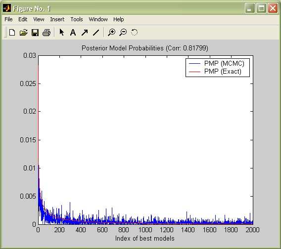
Moreover, reconsider 'Corr PMP' from the summary statistics: for the best 2,000 models, the correlation between their analytical likelihoods and their MCMC frequencies is 0.81. Despite the few iterations, the MCMC sampler seems to have converged reasonably well.
Note that the coefficients reported above were based on MCMC frequencies, while many authors such as FLS prefer statistics based on analytical likelihoods. In order to report coefficients according to these 'exact' posterior model probabilities, type the following:
coef_bma(bmstemp,true)
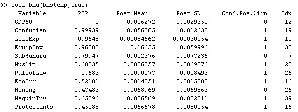
The results differ a bit, since the low number of sampling iterations means that the MCMC results are not perfect. However, they resemble the statistics based on MCMC frequencies.
Posterior Model Probabilities
Reconsider the aggregate statistics such as produced by the command summary_bma(bmstemp);: The posterior expected model size ('Mean no. regressors') is 10.6, rather small compared to the prior expected model size of 41/2=20.5 implied by the uniform model prior. A call to the function plotModelsize plots the posterior vs. the prior model size distribution:
plotModelsize(bmstemp);
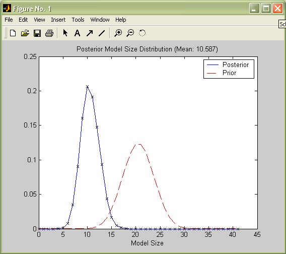
Updating the prior expected model size distribution (implied by the model prior) with the data resulted into a posterior model size distribution that is considerably tilted toward smaller model sizes.
The posterior statistics imply that on average, only 10 to 11 variables are important, in particular those with a high posterior inclusion probability (PIP). The function image_bma allows to check graphically which ones are included in the 'best' models with the highest model probabilities. For simplicity, let us just display the best 50 models:
image_bma(bmstemp);
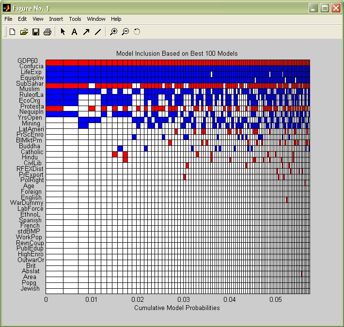
The coefficients are on the y-axis, ordered by their PIP (this can be changed according to the options described in help image_bma) vs the models on the x-axis, as well ordered by importance. The coloured boxes show which variables are included in which model. The best model, to the very left, includes the 10 most covariates with the highest PIP, with initial GDP (GDP60), the sub-Saharan (SubSahar) and the Protestant dummy (Protesta) entering with negative signs (They are coloured in red) - whereas all the other variables enter with positive signs (blue). However, this best model commands less than a half percent of posterior model mass.
Nonetheless the variables seem to keep their signs over the models where they are included.
Posterior Coefficient Densities
In addition to posterior expected values, one might look further into the actual posterior distribution of coefficients. For instance, in their article, Fernández, Ley and Steel report density plots for several variables, e.g. Non-Equipment Investment (NequipInv): With a PIP of 0.45, this variable has a expected posterior coefficient of 0.026 under the 'exact' results reported by coef_bma(bmstemp,true);. This model-weighted average includes the models' coefficients as well as zero in 55% of the cases where it was not included.
I.e. the expected conditional coefficient (the average over the 45% models where it was included) is 0.027/0.45 = 0.06. This is the expected value of the coefficient's conditional posterior distribution produced by the following command:
density_bma(bmstemp,39);
(The number 39 is the index of the variable NequipInv as reported in the last column of the coef_bma(bmstemp) output.)
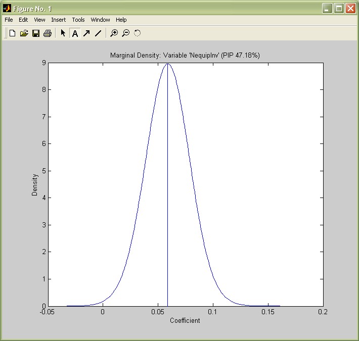
The density plot matches the one by FLS (p.10) quite well and shows that Non-equipment Investment has nearly always positive coefficient, varying about symmetrically around 0.06.
Advanced Topics
Session Saving
In order to save a workspace with 'bma objects', do not forget to save the underlying R workspace as well - otherwise these bma objects become unusable. For example, save what was produced so far to the files 'tutorial.mat' (for the Matlab 'pointers') and 'tutorial.RData' (for the R part):
save 'tutorial';
saveRworkspace 'tutorial';
A such-saved workspace might be loaded again with the command loadRworkspace.
Processing BMA Output
In this tutorial, nearly all functions were used without output arguments, which induced them to present their output in its 'nicest' form.
But requiring an output argument leads to numeric output for all functions involved. For instance try the following to plot the prior model size:
aa=plotModelsize(bmstemp);
plot(aa(:,1))
All other functions produce output in a similar manner.
Additional Documentation
In addition to this tutorial, the function's help comments elaborate on other options and lesser functions: E.g. the above functions might be done with standardized coefficients as explained by:
help density_bma
Since in terms of usability, the BMS Toolbox functions are quite similar (though limited) to the ones of the original R package, the documentation intended for R might help further:
- The online help files for the R package describe the functionality in more detail.
- A pdf tutorial provides a more detailed introduction for users with limited experience in BMA.